Variational autoencoders are unsupervised generative models.
- By “unsupervised”, we mean that they train with unlabeled data.
- By generative, we mean that the variational autoencoders are capable of generating new data which are not in their training set.
The basic steps to construct a geneative model are:
- Collect an unlabeled training set $x_1, x_2, \ldots, x_N$.
- Create a pdf which assigns a high probability to the region of the space from where the elements of the training set are coming from. This will naturally lower the probability of other regions.
- Sample from this pdf to generate new data. This new data will be similar to the data in the training set but will not be one of them.
Before going on explaining Variational autoencoders, we have to explain latent variable models.
Latent variable models
Latent variable models assume the existence of a lower dimensional space, called the “latent space”, which summarizes the data set. In other words, there exist a pdf $p(x|z)$, where $x$ is a point in the data set space and $z$ is a point in the latent space. The relation between $x$ and $z$ is generally constructed by using a neural network.
Example: Assume that we have a list of persons with name, age, height and weight information. Then we have somewhat lost the name and age column, and left with only the height and weight columns. Here is a plot of this data:
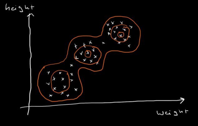
Can we guess which (weight,height) pair in the above plot comes from one of the three classes?
- An adult male
- An adult female
- A child
Note that the data above naturally clusters into three groups. This shows that the space (class, age, height) is actually not three dimensional and if we are given one or two of them, we can get a pretty good idea about the third. This indicates that the real information is concentrated in a lower dimensional region of the three dimensional space. It is this that allow us to make predictions from partial data.
In the example above, the latent space consists of a set of three points, $\{z_1=\mathrm{adult-male}, z_2=\mathrm{adult-female}, z_3=\mathrm{child}\}$. Hence to compute the probability of a given height+weight pair (represented by $x$) is
\begin{eqnarray}
p(x) = \sum_{i=1}^3 p(x|z_i)p(z_i)
\end{eqnarray}
The reverse relation (inference) $p(z|x)$ is much harder to compute.
Note that each $x$ can come from all $z_i$’s.
In image processing, it is much harder to describe what the latent variables correspond to. But, because each pixel value can be predicted using the neighbouring pixels, and various parts of the image can be inferred from other parts, one can see that the lower dimensional latent space exist.
A good guess for a latent space underlying images is the verbal description of image. An 256x256x3=196,608 byte image can be described by a 1000 character = 1000 byte text.
We can make part of the image independent of other parts conditioned on latent variables.
Generative modelling with latent space
To generate new data (ie, images), we need to sample $p(x)$, where x is a data point. İf we have a latent space, this is a two-step process:
- Sample $z \sim p(z)$.
$p(z)$ is assumed to be known to the full. Throughout this article, we will take it to be standard normal, ie, $p(z)=\mathscr{N}(z,0,1)$. $p(z)$ is chosen to be a peaked distribution, as we want to push the points in the latent space close together. The reason for this will be explained later.
Sometimes $p(z)$ is also optimized/learned. This approach is called “learning the prior”. We will not discuss this approach. - Sample $x \sim p_{\theta}(x|z)$
True to the form of parametric estimation theory, the functional form of $p_{\theta}(x|z)$ is assumed to be known, but the parameters $\theta$ is not known and have to be estimated.
In nearly all situations, $p_{\theta}(x|z)$ is implemented as follows:
— The mapping from $z$ to $x$ is achieved by a neural network with weights $\theta$, $x=NN_{\theta}(z)$.
— The probability of $x$ given $z$ is computed by using a gaussian $p_{\theta}(x|z) = \mathscr{N}(x,\mu,I) = \mathscr{N}(x,NN_{\theta}(z),I)$. The variance of this gaussian can be chosen as $I$.
Training is done via ML algorithm: We consider the data points $x_i$ independent of each other and we arrange the parameters $\theta$ such that the probability of the training set is maximized
\begin{eqnarray}
\underset{\theta}{\mathrm{max}} \,\, p_{\theta}(x_1)p_{\theta}(x_2) \ldots p_{\theta}(x_N) = \underset{\theta}{\mathrm{max}} \, \prod_{i=1}^N p_{\theta}(x_i)
\end{eqnarray}
Because we prefer to work with sums, we take the logarithm
\begin{eqnarray}
\underset{\theta}{\mathrm{max}} \, \log \left( \prod_{i=1}^N p_{\theta}(x_i) \right) = \underset{\theta}{\mathrm{max}} \sum_{i=1}^N \log p_{\theta}(x_i)
\end{eqnarray}
recalling Bayes’ law
\begin{eqnarray}
p_{\theta}(x_i) &=& \sum_z p_{\theta}(x_i | z) p(z)
\end{eqnarray}
we arrive at the main object for optimization
\begin{eqnarray}
\underset{\theta}{\mathrm{max}} \sum_{i=1}^N \log \sum_z p_{\theta}(x_i|z)p(z)
\end{eqnarray}
The objective above can be evaluated in two ways:
- If $z$ can only take a small set of values, exact objective can be calculated
- Otherwise, do sampling.
We will investigate alternative (2) below. While we are at it, we will also review the theory of importance sampling. We will examine three scenarios in succession:
Scenario 1: Sampling
To evaluate the above formula, we draw a single sample $z_i \sim p(z)$ for each $x_i$ and evaluate
\begin{eqnarray}
\underset{\theta}{\mathrm{max}} \sum_{i=1}^N \log \sum_z p_{\theta}(x_i|z)p(z) \sim \underset{\theta}{\mathrm{max}} \sum_{i=1}^N \log p_{\theta}(x_i|z_i)\quad,\quad z_i \sim p(z)
\end{eqnarray}
Unfortunately, this will not work, as in most cases $z_i$ and $x_i$ is not related, and $p(x_i|z_i) \approx 0$. This will make the sampling grossly inefficient, and the convergence xill be very slow.
Scenario 2: Importance Sampling
Importance sampling is a very general technique of statistics used in many fields. It is mostly used to cure the problem described above. To understand this problem better, consider the figure below, where $p(x)$ and $r(x)$ are pdf’s.
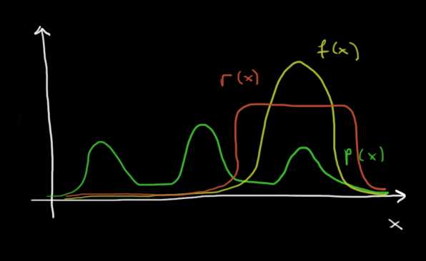
We want to evaluate the expectation by using $N$ samples:
\begin{eqnarray}
\int_{-\infty}^{\infty} f(x)p(x)dx \sim \sum_{i=1}^N f(x_i) \qquad x_i \sim p(x)
\end{eqnarray}
One can immediately see that $p(x)$ is not a good pdf to sample to evaluate the above expectation. 2/3 of the samples will come from the two rightmost humps of $p(x)$, where $f(x)$ is approximately zero. These samples will contribute nothing to the sum. On the other hand, one can see that $r(x)$ is an excellent pdf to sample. All samples will come from the region where $f(x)p(x)$ is significant, hence will contribute to the sum. Can we do a trick which allow us to sample $r(x)$ rather than $p(x)$ to evaluate the sum? The answer is yes:
\begin{eqnarray}
\int_{-\infty}^{\infty} f(x)p(x)dx = \int_{-\infty}^{\infty} \frac{r(x)}{r(x)}f(x)p(x)dx = \sum_{i=1}^N \frac{f(x_i)p(x_i)}{q(x_i)} \qquad x_i \sim q(x)
\end{eqnarray}
Again we emphasize that for this trick to work $q(x) \sim f(x)p(x)$.
Returning back to our unsupervised learning problem, we have
\begin{eqnarray}
\underset{\theta}{\mathrm{max}} \sum_{i=1}^N \log \sum_z p_{\theta}(x_i|z)p(z) \sim \underset{\theta}{\mathrm{max}} \sum_{i=1}^N \log \frac{ p_{\theta}(x_i|z_i) p(z_i)}{r(z_i)}\quad,\quad z_i \sim r(z)
\end{eqnarray}
What is the suitable $r(z)$? According to our previous discussion, $r(z) \sim p_{\theta}(x_i|z_i) p(z_i)$. But the RHS is not suitable for sampling, as it is not a pdf in z. Hence, we write it as $r(z) \sim p_{\theta}(x_i|z_i) p(z_i)=p_{\theta}(z_i|x_i) p(x_i) \sim p_{\theta}(z_i|x_i)$. To summarize, the optimal $r(x)$ to sample is
\begin{eqnarray}
r(z_i) = p_{\theta}(z_i|x_i)
\end{eqnarray}
Unfortunately again, this will not work in most of the cases, as $p_{\theta}(z_i|x_i)$ is not easily computable.
Scenario 3: ELBO (Expectation lower bound)
Using Bayes’ law
\begin{eqnarray}
\log p_{\theta}(x_i) &=& \log \frac{ p_{\theta}(x_i | z) p(z)}{ p_{\theta}(z | x_i)}\\
&=& \log \frac{ p_{\theta}(x_i | z) p(z) r(z)}{ p_{\theta}(z | x_i) r(z)}\\
&=& \log \frac{ p_{\theta}(x_i | z) p(z) r(z)}{ p_{\theta}(z | x_i) r(z)}
\end{eqnarray}
Note that the LHS, and therefore the RHS of the equation is independent of $z$, hence we can take the expectation of the RHS with respect to $r(z)$
\begin{eqnarray}
&=& \int_{z=-\infty}^{\infty} r(z) \log \frac{ p_{\theta}(x_i | z) p(z) r(z)}{r(z) p_{\theta}(z | x_i) r(z)} dz\\
&=& \int_{z=-\infty}^{\infty} r(z) \log \frac{ p_{\theta}(x_i | z) p(z) }{ r(z)}dz + \int_{z=-\infty}^{\infty} r(z) \log \frac{r(z)}{ p_{\theta}(z | x_i) }dz\\
&=& \log \frac{ p_{\theta}(x_i | z_i) p(z_i)}{ r(z)} + \mathrm{KL}(r(z)||p_{\theta}(z | x_i)) \quad \quad z_i \sim p(z)
\end{eqnarray}
Let us rewrite the result of our calculations
\begin{eqnarray}
\log p_{\theta}(x_i) &=& \log \frac{ p_{\theta}(x_i | z_i) p(z_i)}{ r(z_i)} + \mathrm{KL}(r(z)||p_{\theta}(z | x_i)) \quad \quad z_i \sim p(z)
\end{eqnarray}
The first term at the RHS of this equation is known as ELBO. So,
\begin{eqnarray}
\log p_{\theta}(x_i) &=& \mathrm{ELBO} + \mathrm{KL}(r(z)||p_{\theta}(z | x_i)) \quad \quad z_i \sim p(z)
\end{eqnarray}
Note the three facts about this equation:
- LHS of the equation, $\log p_{\theta}(x_i)$, is independent of $r(z)$
- Everything in the ELBO term, ie, $p_{\theta}(x | z)$, $p(z)$ and $q(z)$ are known
- the term $\mathrm{KL}(r(z)||p_{\theta}(z | x_i))$ is not known, as it contains the notorious inference term $p_{\theta}(z | x_i)$. But we know that this term is nonnegative as it is a KL distance.
This gives us a way to pick the optimal $r(z)$: if we pick $r(z)$ in a way to maximize the ELBO term, the KL distance will be minimized, and we will have optimal sampling. Note that the KL distance will never be zero, as $r(z)$ is generally choosen to be a gaussian and $p_{\theta}(z | x_i)$ is a very complicated distribution. But this method will find the closest gaussian to $p_{\theta}(z | x_i)$.
Amortized analysis
It is easy to see that each $x_i$ must have its own sampling distribution $r(z)$, as we want $r(z)$ to approach $p_{\theta}(z | x_i)$ for each $x_i$. Therefore, from now on we will write $r(z|x)$ rather than $r(z)$
To realize $r(z|x)$, we will follow these steps
- We will assume that $r(z|x)$ is a gaussian, $r(z|x)=\mathbb{N}(z,\mu,\sigma)$, where $\mu$ and $\sigma$ are functions of $x$, ie, $\mu=\mu(x)$ and $\sigma=\sigma(x)$
- A neural net takes $x$ as input and generates $\mu(x)$ and $\sigma(x)$ as output. As the neural net has trainable weights denoted by $\varphi$, we will further write these as $\mu_{\varphi}(x)$ and $\sigma_{\varphi}(x)$.
- A $z$ compatible with the given $x$ is sampled from $\mathbb{N}(z,\mu_{\varphi}(x),\sigma_{\varphi}(x))$.
- The training for $\varphi$ is done by maximizing the ELBO term.
Stochastic Gradient optimization of VLB
To summarize, we problem at our hand is
\begin{eqnarray}
\mathrm{Dataset} &:& \quad \{x_1,\ldots,x_n\} \\
\mathrm{optimize} &:& \quad\underset{\theta, \varphi}{\mathrm{max}} \sum_{i=1}^n \underset{z \sim r_{\varphi}(z|x)}{\mathrm{E}} \log \frac{p_{\theta}(x,z)}{r_{\varphi}(z|x)}
\end{eqnarray}
And we need to do the optimization wrt $\theta$ and $\varphi$. Consider a single term in the above sum:
\begin{eqnarray}
\nabla_{\theta, \varphi} \underset{z \sim r_{\varphi}(z|x_i)}{\mathrm{E}} [\log p_{\theta}(x_i,z) -\log r_{\varphi}(z|x_i)]
\end{eqnarray}
Let us concentrate on the gradient wrt $\theta$
\begin{eqnarray}
\nabla_{\theta} \underset{z \sim r_{\varphi}(z|x_i)}{\mathrm{E}} [\log p_{\theta}(x_i,z)-\log r_{\varphi}(z|x_i)] &=& \underset{z \sim r_{\varphi}(z|x_i)}{\mathrm{E}} \nabla_{\theta} \log p_{\theta}(x_i,z) \\
&\sim& \nabla_{\theta} \log p_{\theta}(x_i,z) \qquad z \sim r_{\varphi}(z|x_i)
\end{eqnarray}
In the second step we performed SGD by approximating the expectation with a single sample.
Gradient wrt $\varphi$ is not as easy, as in this case gradient cannot jump over the expectation. So we write the expectation in full in this case
\begin{eqnarray}
\nabla_{\varphi} \underset{z \sim r_{\varphi}(z|x_i)}{\mathrm{E}} [\log p_{\theta}(x_i,z)-\log r_{\varphi}(z|x_i)] & \neq & \underset{z \sim r_{\varphi}(z|x_i)}{\mathrm{E}} \nabla_{\varphi} [\log p_{\theta}(x_i,z)-\log r_{\varphi}(z|x_i)]
\end{eqnarray}
Remember that
\begin{eqnarray}
r_{\varphi}(z|x_i) = \mathbb{N}(z,\mu_{\varphi}(x_i),\sigma_{\varphi}(x_i))=\mu_{\varphi}(x_i) + \sigma_{\varphi}(x_i) .\mathbb{N}(z,0,1)
\end{eqnarray}
Hence given $x$, $z$ can be estimated by a single sample
\begin{eqnarray}
z = \mu_{\varphi}(x_i) + \sigma_{\varphi}(x_i).n \qquad n\sim \mathbb{N}(z,0,1)
\end{eqnarray}
If this is substituted, the $\varphi$ dependence of the sampling distribution is eliminated and $\nabla_{\varphi}$ can jump over the expectation:
\begin{eqnarray}
\nabla_{\varphi} \underset{n \sim \mathbb{N}(z,0,1)}{\mathrm{E}} [\log p_{\theta}(x_i,z)-\log r_{\varphi}(z|x_i)] & = & \underset{n \sim \mathbb{N}(z,0,1)}{\mathrm{E}} \nabla_{\varphi} [\log p_{\theta}(x_i,z)-\log r_{\varphi}(z|x_i)] \\
& \sim & \nabla_{\varphi} [\log p_{\theta}(x_i,z)-\log r_{\varphi}(z|x_i)] \qquad n \sim \mathbb{N}(z,0,1)
\end{eqnarray}
In the second line, we have estimated the gradient of the expectation with a single sample, and it can be easily seen that this is an unbiased estimate.
===============================================
Importance Weighted Autoencoder (IWAE)
To evaluate the above formula, we sample $p(z)$ $K$ times for each $x_i$ to generate samples $z_i^{(k)} \sim p(z)$ and evaluate
\begin{eqnarray}
\underset{\theta}{\mathrm{max}} \sum_{i=1}^N \log \sum_z p_{\theta}(x_i|z)p(z) \sim \underset{\theta}{\mathrm{max}} \sum_{i=1}^N \log \frac{1}{K} \sum_{k=1}^K p_{\theta}(x_i|z_i^{(k)})\quad,\quad z_i^{(k)} \sim p(z)
\end{eqnarray}
The problem with this is that $p(z)$ may not be the best function to sample to evaluate $p(x|z)$, as the $z$s we sample may not be the ones that result in $x$. This results in slow convergence. So, we will rather sample from an another distribution $z_i^{(k)} \sim q(z)$, whose properties we dont know yet, which we hope will give a faster convergence.
\begin{eqnarray}
\underset{\theta}{\mathrm{max}} \sum_{i=1}^N \log \sum_z p_{\theta}(x_i|z)p(z) &=& \underset{\theta}{\mathrm{max}} \sum_{i=1}^N \log \sum_z \frac{q(z)}{q(z)} p_{\theta}(x_i|z)p(z) \\
&\sim& \underset{\theta}{\mathrm{max}} \sum_{i=1}^N \log \frac{1}{K} \sum_{k=1}^K \frac{p(z_i^{(k)})}{q(z_i^{(k)})}p_{\theta}(x_i|z_i^{(k)})\quad,\quad z_i^{(k)} \sim q(z)
\end{eqnarray}
How to choose the best $q(z)$ for a given $x_i$? The theory of importance sampling says that $q(z)$ works best when it is proportional to $p(z)p_{\theta}(x_i|z)$, or, $p_{\theta}(z|x_i)$,
\begin{eqnarray}
q_i(z) &\propto& p(z)p_{\theta}(x_i|z) \\
&=& p_{\theta}(z|x_i)p_{\theta}(x_i) \\
&\propto& p_{\theta}(z|x_i)
\end{eqnarray}
(When passing from line 2 to line 3 above, we can ignore $p_{\theta}(x_i)$, as it is not a function of $z$ and hence only acts as a scaling factor.)
Therefore we have to choose $q(z)$ as close as possible to $p_{\theta}(z|x_i)$. But, this implies that for each $x_i$ we must have a different $q(z)$. Notationally, we indicate such $q(z)$ corresponding to $x_i$ with $q_i(z)$. Now the samples $z_i^{(k)}$ is drawn from $q_i(z)$. Note that if we consider $x_i$ as images, this means that each image $x_i$ will have a separate $q_i(z)$ trained for itself.
The closeness between $q_i(z)$ and $p_{\theta}(z|x_i)$ can be established by minimizing the KL distance $\mathrm{KL}(q_i(z)||p_{\theta}(z|x_i))$. One way of making this distance small is
- For each $x_i$, choose a $q_i(z)$ which is an easy to work with parametrized distribution, say a gaussian.
\begin{eqnarray}
q_i(z) = \mathscr{N}( z; \mu_i, \sigma_i )
\end{eqnarray} - Find the parameters $ \mu_i, \sigma_i$ by minimizing the distance
\begin{eqnarray}
\underset{\mu_i, \sigma_i}{\mathrm{min}} \quad \mathrm{KL}(q_i(z)||p_{\theta}(z|x_i)).
\end{eqnarray}
Unfortunately, we generally do not know what $p_{\theta}(z|x_i)$ is. What we know is $p_{\theta}(x_i |z)$, which is a combination of neural net ($(x_i |z)$ part) and a gaussian ($p(.)$ part). It is not possible to invert this. But there is a mathematical trick to sidetrack this difficulty.
\begin{eqnarray}
\underset{\mu_i, \sigma_i}{\mathrm{min}} \quad \mathrm{KL}(q_i(z)||p_{\theta}(z|x_i)) &=& \underset{\mu_i, \sigma_i}{\mathrm{min}} \quad q_i(z)\left[ \log q_i(z) -\log p(z)-\log p_{\theta}(x_i|z)] + \log p_{\theta}(x_i)\right] \\
&=& \underset{\mu_i, \sigma_i}{\mathrm{min}} \left[ \underset{z\sim q_i(z)}{\mathrm{E}}\left[ \log q_i(z) -\log p(z)-\log p_{\theta}(x_i|z) \right] + \underset{z\sim q_i(z)}{\mathrm{E}} \log p_{\theta}(x_i)\right]
\end{eqnarray}
Note that
\begin{eqnarray}
\underset{z\sim q_i(z)}{\mathrm{E}} \log p_{\theta}(x_i) = \log p_{\theta}(x_i)
\end{eqnarray}
so this term is independent of $\mu_i$ and $\sigma_i$ and hence does not contribute to minimization. Therefore we remove it. The resulting target for optimization is
\begin{eqnarray}
\underset{\mu_i, \sigma_i}{\mathrm{min}} \quad \left[ \log q_i(z) -\log p(z)-\log p_{\theta}(x_i|z) \right] \qquad z \sim q_i(z)
\end{eqnarray}
and all the terms here are known.
The above discussion for IWAE results in the following algorithm:
- consider $q_i(z)$ as a gaussian and pick arbitrary initial $\mu_i$, $\sigma_i$. Also, pick arbitrary initial $\theta$ for $p_{\theta}(x_i|z)$. Consider $p(z)$ as a gaussian with mean zero and variance 1.
- For each $x_i$, sample $q_i(z)$ $K$ times, to obtain $z_i^{(k)}$.
- evaluate
\begin{eqnarray}
\sum_{i=1}^N \log \frac{1}{K} \sum_{k=1}^K \frac{p(z_i^{(k)})}{q_i(z_i^{(k)})}p_{\theta}(x_i|z_i^{(k)})\quad,\quad z_i^{(k)} \sim q_i(z)
\end{eqnarray} - Do a gradient ascent along $\theta$’s. Find new $\theta$’s.
- For each $i$, do a gradient descent along $\mu_i$, $\sigma_i$ on the cost function
\begin{eqnarray}
\quad \left[ \log q_i(z) -\log p(z)-\log p_{\theta}(x_i|z) \right]
\end{eqnarray}
Find new $\mu_i$, $\sigma_i$ for $q_i(z)$. Use $z = z_i^{(k)}$ in the cost function. - Goto 2 untill convergence occurs.
Amortized analysis for IWAE
In the section above we have assigned a gaussian $p_i(z)= \mathscr{N}( z; \mu_i, \sigma_i )$ to each data point/image $x_i$ for efficient sampling in latent space. $\mu_i$ and $\sigma_i$ of each of these gaussians must be found through gradient descent.
There is a different way of finding $\mu_i$ and $\sigma_i$ for a given data point/image $x_i$: we can design a neural net which computes $\mu_i, \sigma_i$ for any given data point/image $x_i$.
\begin{eqnarray}
q_{\phi}(z|x_i) = \mathscr{N}( z; \mu_{\phi}(x_i), \sigma_{\phi}(x_i) )
\end{eqnarray}
where $\mu_{\phi}(x_i)$ and $\sigma_{\phi}(x_i)$ represents a single neural network whose weights and biases are represented by $\phi$. Sampling from this system is done in two steps:
- The data point/image $x_i$ is fed as an input into the neural network. The output of the neural network is $\mu_i=\mu_{\phi}(x_i)$ and $\sigma_i= \sigma_{\phi}(x_i)$.
- Form the gaussian $\mathscr{N}(z,\mu_i, \sigma_i)$.
- Sample from this gaussian: $\mu_i+\epsilon \sigma_i$ where $\epsilon \sim\mathscr{N}(0,I)$ .
Hence we can modify the above 6-step training algorithm as follows:
- initialize $\theta$ and $\phi$.
- Fed all $x_i$ into the neural network $\mu_i=\mu_{\phi}(x_i)$, $\sigma_i=\sigma_{\phi}(x_i)$ to find $(\mu_i, \sigma_i)$ for each one of them.
- Sample $q_{\phi}(\mu_i, \sigma_i)$ $K$ times to find $z_i^{(k)}$.
- Use $x_i$ and $z_i^{(k)}$ to evaluate
\begin{eqnarray}
\sum_{i=1}^N \log \frac{1}{K} \sum_{k=1}^K \frac{p(z_i^{(k)})}{q_i(z_i^{(k)})}p_{\theta}(x_i|z_i^{(k)})\quad,\quad z_i^{(k)} \sim q_i(z)
\end{eqnarray} - Do a gradient ascent along $\theta$’s. Find new $\theta$’s.
- Do a gradient descent along $\phi$ on the cost function
\begin{eqnarray}
\quad \left[ \log q_{\phi}(z) -\log p(z)-\log p_{\theta}(x_i|z) \right]
\end{eqnarray}
to find new $\phi$ for $q_{\phi}(z)$. - Goto 2 untill convergence occurs.
Classic VAE
Above we considered IWAE. We will also illustrate the classical autoencoder, as they are used very frequently. We will give two different proofs:
Proof 1: Via Jensen inequality.
The input of this neural network is $x$. The output of the neural net is $\mu_{\phi}(x)$ and $\sigma_{\phi}(x)$. Then we can sample a $z$ using a gaussian with $\mu_{\phi}(x)$ and $\sigma_{\phi}(x)$.
As we want $q_{\phi}(z|x)$ to be as close as possible to $p_{\theta}(z|x)$. Taking $K=1$ above and $N=1$ we can show that
\begin{eqnarray}
\log p_{\theta}(x) = [ \log p_{\theta}(x|z) + \log p(z) – \log q_{\phi}(z|x) ] + \mathrm{KL}(q_{\phi}(z|x) || p_{\theta}(z|x) )
\end{eqnarray}
The bracketed quantity immediately to the right of the equality is known as ELBO (evidence lower bound) or VLB (variational lower bound). Hence we can rewrite the equation as
\begin{eqnarray}
\log p_{\theta}(x) = ELBO(x,\theta,\phi) + \mathrm{KL}(q_{\phi}(z|x) || p_{\theta}(z|x) )
\end{eqnarray}
- Consider increasing ELBO by changing $\phi$. $\log p_{\theta}(x)$ is not a function of $\phi$, hence it will remain constant. This means KL distance between $q_{\phi}(z|x)$ and $p_{\theta}(z|x)$ will decrease and we will generate better samples.
- Consider increasing ELBO by changing $\theta$. In this case either $p_{\theta}(x)$ will increase, or the KL distance will decrease, or both.
How to find the best mean and variance? We want to minimize the KL distance between $q_{x_i}(z)$ and $p(z|x)$:
\begin{eqnarray}
\underset{q_{x_i}(z)}{\mathrm{min}} \; \mathrm{KL} ( q_{x_i}(z) || p_{\theta}(z|x) ) &=& \underset{q_{x_i}(z)}{\mathrm{min}} \;\; \underset{z \sim q_{x_i}(z)}{\mathrm{E}} \mathrm{log} \left( \frac{q_{x_i}(z)}{p_{\theta}(z|x) } \right) \\
&=& \underset{q_{x_i}(z)}{\mathrm{min}} \;\; \underset{z \sim q_{x_i}(z)}{\mathrm{E}} \left[ \log q_{x_i}(z) – \log p(z) -\log p_{\theta}(x|z) \right]+\log p_{\theta}(x_i)
\end{eqnarray}
The second term in the above equation is defined as ELBO
\begin{eqnarray}
\mathrm{ELBO} = -E[\left[ \log q_{x_i}(z) – \log p(z) -\log p_{\theta}(z|x) \right]]
\end{eqnarray}
Rearranging
\begin{eqnarray}
\log p_{\theta}(x_i) = ELBO + \mathrm{KL} ( q_{x_i}(z) || p_{\theta}(z|x) )
\end{eqnarray}
Note that both $\log p_{\theta}(x_i)$ and $\mathrm{KL} ( q_{x_i}(z) || p_{\theta}(z|x) )$ are by definition positive. Hence maximizing ELBO over $q_{x_i}(z)$ will necessarily minimize the KL distance, and make $q_{x_i}(z)$ a better choice for sampling. But also note that the KL distance will never be zero, as we choose $q_{x_i}(z)$ to be gaussian and $\mathrm{KL} ( q_{x_i}(z) || p_{\theta}(z|x) )$ is not necessarily gaussian, so there will always be some distance between the two. This is not very important, as importance sampling will work for any $q(z)$.
All terms in ELBO are known and easy to calculate ( $\log q_{x_i}(z)$ and $\log p(z)$ are choosen to be gaussians. $\log p_{\theta}(z|x)$ is a neural network + a gaussian. SGD on $\mu(x)$ and $\sigma(x)$ can be run on ELBO because it is an expectation.
Amortized Analysis
In the formulation above, for each $x_i$ we have to optimize a separate $q_{x_i}(z)$. If $x_i$ is an image, this means that we have to find a separate $q_{x_i}(z)$ for each image separately. We can amortize this process by a Neural network. In more concrete terms, rather than optimizing
\begin{eqnarray}
\mathrm{KL} ( q_{x_i}(z) || p_{\theta}(z|x) )
\end{eqnarray}
we will try to optimize
\begin{eqnarray}
\mathrm{KL} ( q_{\phi}(z|x) || p_{\theta}(z|x) )
\end{eqnarray}
$q_{\phi}(z|x)$ is a neural network which wşll generate $\mu(x)$ and $\sigma(x)$ for a given image $x$. So we have
\begin{eqnarray}
p_{\theta}(x|z) = \mathscr{N}( x-NN_{\theta(z)}, I) \\
q_{\phi}(z|x) = \mathscr{N}( \mu_{\phi}(x), \sigma_{\phi}(x) )
\end{eqnarray}
Sampling from $q_{\phi}(z|x)$ will be done by $z=\mu(x)+\epsilon \sigma(x)$ where $\epsilon \sim \mathscr{N}(0,1)$. There will be no need to sample from $p_{\theta}(x|z)$. Therefore, we modify our formula for ELBO above as
\begin{eqnarray}
\mathrm{ELBO} = E[\left[ \log q_{\phi}(z|x) – \log p(z) -\log p_{\theta}(z|x) \right]]
\end{eqnarray}
General theory of optimization
===============================================
Here
- $p(x|z)$ is essentially a deterministic pdf which corresponds to decoder neural network. $p(x|z)=\delta(x-d(z)).$
- $p(z)$ determines how the input to the decoder is distributed. We arbitrarily set this to standard normal distribution, ie, $z \sim N(0,1)$ as we want to push the latent space representation of objects together. After this choice, all $z$’s will come from within a narrow sphere with a high probability.
- $p(z|x)$ is the inverse function of the neural network. As the neural net is not guaranteed to be bijective, this relation is not deterministic in general. In most cases, it is not possible to get an analytic expression for it.
We will try to estimate $p_{\theta}(z|x)$ by an another neural network, $q_{\phi}(z|x)$. To introduce
\begin{eqnarray}
&=& \underset{z \sim p_{\theta}(z|x)}{E} \log \left( \frac{p_{\theta}(x|z)p(z)}{p(z|x)} \frac{q_{\phi}(z|x)} {q_{\phi}(z|x)} \right)
\end{eqnarray}
Armed with the knowledge of latent spaces, we can modify the method of sampling from a generative model as follows.
- Sample a z from the latent space
- Reconstruct the new data point x by $x=f(z)$
Given the training set $x_1, x_2, \ldots, x_N$ and a parametric family of pdf’s $p_{\theta}(x)$, we want to find the $\theta^*$ which maximizes the probability of this training set within the family:
$$\theta^*=\underset{\theta}{\mathrm{argmax}} \prod_{i=1}^{N}p(x_i)
= \underset{z \sim q_{\phi}(z|x)}{E} \log \eft( \frac{p_{\theta}(x|z)}{p(z)} \right)$$
========================
Minimizing $\mathrm{KL}(q_i(z)||p_{\theta}(z|x_i))$ is the same as maximizing $-\mathrm{KL}(q_i(z)||p_{\theta}(z|x_i))$. Hence our cost function is:
\begin{eqnarray}
\underset{\theta,q_i(z)}{\mathrm{max}} \left[ \sum_{i=1}^N \log \frac{1}{K} \sum_{k=1}^K \frac{p(z_i^{(k)})}{q_i(z_i^{(k)})}p_{\theta}(x_i|z_i^{(k)})\; – \; \mathrm{KL}(q_i(z)||p_{\theta}(z|x_i)) \right] \quad,\quad z_i^{(k)} \sim q_i(z)
\end{eqnarray}
If $q_i(z)$ is gaussian, it is maximized by a gradient ascent on its mean and variance. As $q_i(z)$ becomes closer to $p_{\theta}(z|x_i)$ sampling becomes more efficient. Note that this method will work for any $q_i(z)$, but it will require too many samples for convergence if $q_i(z)$ is not optimal.