Time and frequency considerations
It is impossible to read a continuous signal into a computer. Hence, reading a continuous signal always involves some sort of sampling/discretization. And discretization brings some loss of data.
Assume we are sampling data (in our case, sound) with $N$ samples per second. The fastest signal that can be accurately captured with this sampling speed is $\pm N/2$ Hz. Hence if we capture any signal $x(t)$ with a sampling rate of N samples per second, and then take DFT of it and find $X(\omega)$, and then plot it, the frequency axis must go from $-N/2$ Hz to $N/2$ Hz. In a sense, the “sampling rate” and the “bandwidth of the medium” is one and the same thing.
Actually it is not possible to plot $X(\omega)$, as it is a complex signal. We usually plot $|X(\omega)|$ instead.
The following code illustrates the tradeoffs of approximating a continuous signal with a sampled signal. Try it with different sampling rates and see what happens. As long as the sampling rate (fs) is more than twice the frequency of the signal, the fourier transform of the signal is correct. If the sampling rate fells below this limit, strange things happen.
import numpy as np
import matplotlib.pyplot as plt
from numpy.fft import fft, fftfreq, fftshift

fs = 44100  # Sampling rate
freq = 10000
seconds = 1  # Duration of recording
time = np.linspace(0,seconds,fs)
mysignal_in_time = np.cos(2*np.pi*freq*time)

frequencies = np.linspace(-fs/2,fs/2,fs)
mysignal_in_frequency_abs = fftshift(np.abs(fft(mysignal_in_time)))
plt.figure(2)
plt.plot(frequencies, mysignal_in_frequency_abs)

plt.show()
Sound Recording, FT and Modulation
The following code will record sound for 3 seconds and then will plot the sound signal. The channels parameter in the sd.rec function probably determines whether the recording is mono or stereo. As we dont have stereo equipment, we set channels=1.
import numpy as np
import matplotlib.pyplot as plt
from numpy.fft import fft, fftfreq, fftshift
import sounddevice as sd
# recording the sound
fs = 44100 # Sample rate
seconds = 3 # Duration of recording
myrecording = sd.rec(int(seconds * fs), samplerate=fs, channels=1)
sd.wait() # Wait until recording is finished

# display the sound signal
myrecording_in_time = np.squeeze(myrecording)
time = np.linspace(0,seconds,myrecording_in_time.shape[0])
plt.figure(1)
plt.plot(time,myrecording_in_time)

# ft the sound signal and display its magnitude
frequencies = np.linspace(-fs/2,fs/2,fs*seconds)
myrecording_in_frequency_abs = fftshift(np.abs(fft(myrecording_in_time)))
plt.figure(2)
plt.plot(frequencies , myrecording_in_frequency_abs)

#modulate the signal
myrecording_in_time_modulated = np.multiply(myrecording_in_time, np.cos(2*np.pi*10000*time))

plt.figure(3)
plt.plot(time,myrecording_in_time_modulated)

myrecording_in_frequency_modulated_abs = fftshift(np.abs(fft(myrecording_in_time_modulated)))
plt.figure(4)
plt.plot(frequencies , myrecording_in_frequency_modulated_abs)

plt.show()
Modulating two signals together
In the following code, two sound signals is recorded. One is modulated into 5KHz, the other is modulated into 11KHz.
import numpy as np
import matplotlib.pyplot as plt
from numpy.fft import fft, fftfreq, fftshift, ifft
import sounddevice as sd
# recording the sound
fs = 44100 # Sample rate
seconds = 3 # Duration of recording
myrecording = sd.rec(int(seconds * fs), samplerate=fs, channels=1)
sd.wait() # Wait until recording is finished
# display the sound signal
myrecording_in_time_1 = np.squeeze(myrecording)
time = np.linspace(0,seconds,myrecording_in_time_1.shape[0])
plt.figure(1)
plt.plot(time , myrecording_in_time_1)
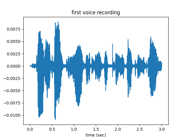
plt.title("first voice recording")
plt.xlabel("time (sec)")
# ft the sound signal and display its magnitude
frequencies = np.linspace(-fs/2,fs/2,fs*seconds)
myrecording_in_frequency_1 = fftshift(fft(myrecording_in_time_1))
plt.figure(2)
plt.plot(frequencies , np.abs(myrecording_in_frequency_1))
plt.title("ft of first voice recording")
plt.xlabel("frequency (Hz)")
xx = input('After pressing return, enter your voice: ')
myrecording = sd.rec(int(seconds * fs), samplerate=fs, channels=1)
sd.wait() # Wait until recording is finished
# display the sound signal
myrecording_in_time_2 = np.squeeze(myrecording)
plt.figure(3)
plt.plot(time ,myrecording_in_time_2)
plt.title("second voice recording")
plt.xlabel("time (sec)")
# ft the sound signal and display its magnitude
myrecording_in_frequency_2 = fftshift(fft(myrecording_in_time_2))
plt.figure(4)
plt.plot(frequencies , np.abs(myrecording_in_frequency_2))
plt.title("ft of second voice recording")
plt.xlabel("frequency (Hz)")
#modulate the signal
myrecording_in_time_modulated_1 = np.multiply(myrecording_in_time_1, np.cos(2*np.pi*5000*time))
plt.figure(5)
plt.plot(frequencies , np.abs(fftshift(fft(myrecording_in_time_modulated_1))))
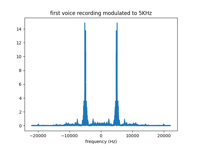
plt.title("first voice recording modulated to 5KHz")
plt.xlabel("frequency (Hz)")
myrecording_in_time_modulated_2 = np.multiply(myrecording_in_time_2, np.cos(2*np.pi*11000*time))
plt.figure(6)
plt.plot(frequencies , np.abs(fftshift(fft(myrecording_in_time_modulated_2))))
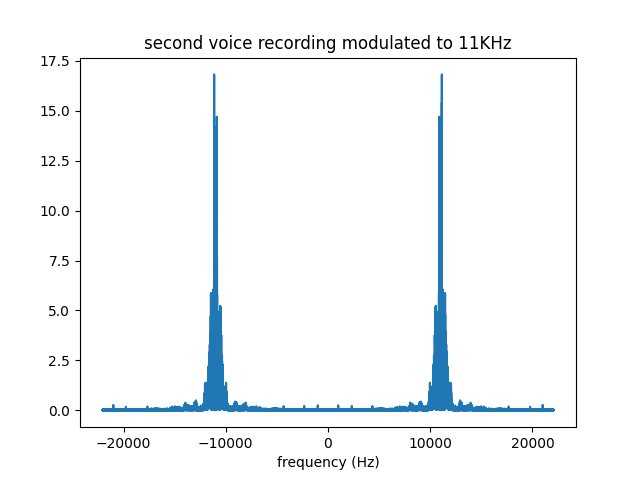
plt.title("second voice recording modulated to 11KHz")
plt.xlabel("frequency (Hz)")
myrecording_in_time_modulated = np.add(myrecording_in_time_modulated_1,myrecording_in_time_modulated_2)
plt.figure(7)
plt.plot(time,myrecording_in_time_modulated)
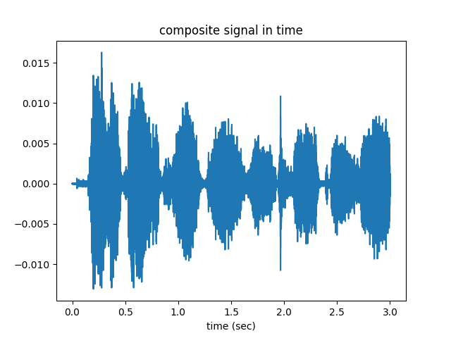
plt.title("composite signal in time")
plt.xlabel("time (sec)")
myrecording_in_frequency_modulated = fftshift(fft(myrecording_in_time_modulated))
plt.figure(8)
plt.plot(frequencies , np.abs(myrecording_in_frequency_modulated))
plt.title("the composite signal in frequency")
plt.xlabel("frequency (Hz)")
Let us discuss how this code works, step by step. To illustrate what we are doing better, we will use two radio stations as an example:
Radio station 1 wants to broadcast some music. Below is a three second recording of the piece they are broadcasting. Call this signal $s_1(t)$
If we look to the same song at the frequency domain, we will see $S_1(\omega)$

Note that $S_1(\omega)$ has a very limited bandwith, ie, it only exists between -3KHz and 3KHz, which is the natural range for human voice and sounds of many musical instruments. Most of the frequency range is empty (ie, zero or close to zero), which hints that the frequencies are underutilized.
Here is the second sound recording, broascasted by Radio station 2. Call this signal $s_2(t)$. Assume that this is an interview with a famous movie star.

In frequency domain, this interview will be seen as $S_1(\omega)$, shown below:
Again, only the frequencies between -3KHz and 3KHz are utilized. The rest is zero.
These two radio stations want to broadcast their signals into the air for their customers to receive them. But if they do this, their signals will “mix” into each other in the air, as both signals overlap, ie, they “live” in the same -3KHz to 3KHz range. Listeners will only receive $s_1(t)+s_2(t)$, and it will not be possible to separate this reception into $s_1(t)$ and $s_2(t)$. (Actually some statistical techniques exist to effect such a separation. One such technique is ICA-independent component analysis. But this is a topic for an another lecture).
The solution to this problem is called “modulation”. As $s_1(t)$ and $s_2(t)$ use only a small proportion of the frequency range, we can combine them into a single signal without mixing them. The way to do this is to “map” (or modulate) these signals into different regions of frequency domain.
We will map $s_1(t)$ to 5KHz. This can be done by multiplying $s_1(t)$ with a 5KHz sinusoid signal, ie, $s_1(t) \rightarrow s_1(t) \cos(2*3.14*5000t)$. The result is shown below, in frequency domain..
We will map $s_2(t)$ to 11KHz. This can also be done by multiplying $s_1(t)$ with a 11KHz sinusoid signal, ie, $s_2(t) \rightarrow s_2(t) \cos(2*3.14*11000t)$. The result is shown below, in frequency domain..
Then these two modulated signals are broadcasted from the antennas of the respective radio stations separately, and they mix up in the air, becoming the “composite signal” $c(t)=s_1(t) \cos(2*3.14*5000t)+s_2(t) \cos(2*3.14*11000t)$. When we look to this signal in time, it seems like it is completely jumbled and mixed up.
But if we take the fourier transform and look to the same signal in frequency, we can see that the individual radio stations did not mix up and stay completely separate from each other..
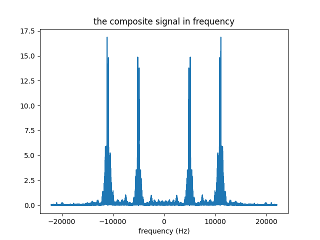
The composite signal above is what our radio set receives. It is a single signal, and it contains the broadcast all the radio stations of that area sitting separate from each other.
Tuning into a radio station
Up till now, we have described what happens in the radio station (ie, the broadcaster) and in the air. Now we have to describe what happens in our radio set. We will not give any code, as this is the 4th question of your final. Excepting the np.print statements, you will be required to write 8-10 lines of python-numpy code in total.
Radio set receives the composite signal. Its first task is to filter out the desired radio station from the composite signal. This is called “tuning into a station”, and is achieved via a bandpass filter.
Below is the plot for the bandpass filter to filter out station 1. For each station, a different bandpass filter must be used.
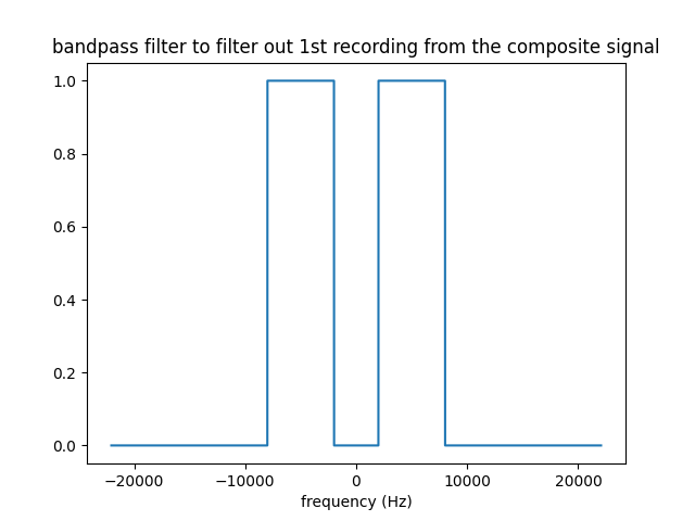
The bandpass filter is centered at the broadcast frequency of the desired radio station and each of its lobes are 6KHz wide. In other words, BP filter is 1 in the frequency range [-f-3KHz, -f+3KHz], [f-3KHz, f+3KHz] and zero elsewhere, where f is the broadcast frequency of the desired radio station.
Station 1 broadcasts at 5KHz, which means that the lobes of the filter are at [-8KHz,-2KHz] to [2KHz, 8KHz].
The bandpas filtering is achieved by multiplying the BP filter and the composite signal in frequency, or convolving them in time. The result (in frequency domain) is shown below.

Next, we have to multiply the BP filtered result with $cos(2 \pi f t)$ in time (or, convolve them in frequency), where $f$ is the broadcast frequency of the desired radio station. The result is shown below, in frequency.

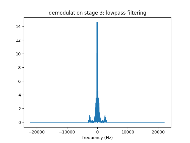
The central lobe is the signal we desire, but we do not want the sidelobes at the $\mp 10KHz$. Hence we pass this signal from a lowpass filter depicted below

Again, filtering is done by multiplication in frequency (or convolution in time). The result is shown below.
When we look at this signal in time, as shown below, we see that we have recovered the signal 1 from the composite signal that we receive from the air.
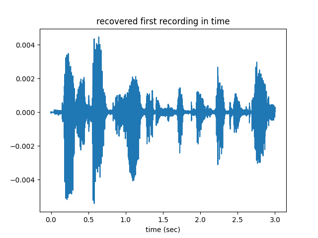
signal from station 2 can be recovered in the same way.